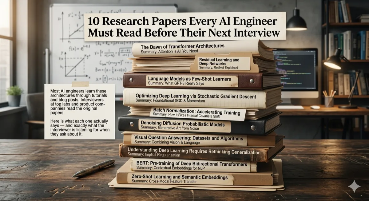
10 Research Papers Every AI Engineer Must Read Before Their Next Interview
Most AI engineers learn architectures through tutorials and blog posts. Interviewers at top labs read the original papers. Here is what each one actually says — and exactly what the interviewer is listening for.
Interview Prep | Research Papers | Machine Learning | March 2026 ~15 min read
The gap between tutorials and interviews
There is a specific type of interview question that separates candidates who have used the technology from candidates who understand it. It usually sounds something like: “Walk me through how multi-head attention works and why we need multiple heads instead of just one.” Or: “Why does LoRA work, mathematically? What is the assumption it makes about weight updates?”
The candidates who answer fluently — not from a tutorial summary, but from actual understanding — almost always share one habit: they read the original papers. Not every word. But enough to understand the actual problem being solved, the key insight, and the design decisions the authors made and why.
The ten papers in this list are the ones that appear most frequently in AI engineering interviews at top companies in 2026. Each entry covers the core idea in plain language, explains why it matters, points to the interview questions it generates, and includes a minimal code sketch to make the concept concrete.
How to use this article: Read the summary. Then open the paper. Then come back and read the interview questions. The summary gives orientation. The paper gives depth. The questions give focus. Doing all three is how engineers walk into interviews and walk out with offers.
01 — Attention Is All You Need: The Transformer
2017 | Vaswani et al. | Google Brain | Difficulty: Medium arXiv:1706.03762
The paper that started everything.
Before 2017, sequence modeling meant RNNs — processing tokens one at a time, left to right. The problem: by the time the model reached token 200, it had mostly forgotten token 3. Vaswani et al. removed recurrence entirely and replaced it with self-attention: every token attends to every other token simultaneously, with no sequential dependency. The result was a model that could be parallelized completely during training and could capture long-range dependencies that RNNs routinely missed.
The key mechanism is scaled dot-product attention: Q (Query), K (Key), and V (Value) matrices are derived from the input. Each token’s query is compared against all keys to produce attention weights, which are then used to compute a weighted sum of the values. Multi-head attention runs this process in parallel across multiple representation subspaces — allowing the model to simultaneously attend to syntactic structure, semantic similarity, and positional relationships rather than collapsing them into a single attention signal.
Why it changed everything: GPT, BERT, T5, Claude, Gemini, and every frontier model built since 2018 is a Transformer variant. Understanding this paper is not optional background — it is the architectural foundation of the entire field.
Interview questions it generates:
- Explain Q, K, V. Why are there three separate matrices instead of one?
- Why divide by sqrt(d_k) in the attention formula? What happens without it?
- What is the difference between encoder-only, decoder-only, and encoder-decoder architectures? Give a model example of each.
- What is positional encoding and why is it necessary? Why not just use integer positions?
- Multi-head vs. single-head attention — what does each head learn?
Scaled dot-product attention — PyTorch:
import torch
import torch.nn.functional as F
import math

def scaled_dot_product_attention(Q, K, V, mask=None):
    """
    Q, K, V: (batch, heads, seq_len, d_k)
    Returns: attention output + weights
    """
    d_k = Q.size(-1)

    # Step 1: compute raw scores — how much does each Q attend to each K?
    scores = torch.matmul(Q, K.transpose(-2, -1)) / math.sqrt(d_k)

    # Step 2: mask future positions (decoder only)
    if mask is not None:
        scores = scores.masked_fill(mask == 0, float('-inf'))

    # Step 3: softmax → attention weights (sum to 1 across keys)
    attn_weights = F.softmax(scores, dim=-1)

    # Step 4: weighted sum of values
    output = torch.matmul(attn_weights, V)

    return output, attn_weights
02 — LoRA: Low-Rank Adaptation of Large Language Models
2021 | Hu et al. | Microsoft | Difficulty: Medium arXiv:2106.09685
Fine-tune a 7B model on a laptop.
Fine-tuning a large model means updating every weight — hundreds of billions of parameters, requiring massive GPU memory and hours of compute. LoRA’s insight: weight updates during fine-tuning are intrinsically low-rank. Instead of updating a large weight matrix W directly, LoRA freezes W and learns two small matrices A and B where the update is delta-W = BA. If W is 1024x1024 and the rank r is 8, LoRA trains two matrices of size 1024x8 and 8x1024 — roughly 99% fewer trainable parameters.
At inference time, the adapters are merged back into the original weights: W’ = W + BA. No additional latency. The merged model is identical in size to the original. LoRA makes fine-tuning accessible on consumer hardware and enables deploying dozens of specialized model variants efficiently — a single base model with swappable adapters.
Why interviewers love it: LoRA is how almost all real-world LLM customization happens today. Any company fine-tuning a model is almost certainly using LoRA or a variant. The math is simple enough to explain precisely, and the design tradeoffs (rank selection, which layers to adapt, merge vs. keep-separate) generate excellent follow-up questions.
Interview questions it generates:
- What is the mathematical justification for why weight updates are low-rank?
- How do you choose rank r? What are the tradeoffs at r=1 vs r=64?
- Why does LoRA add zero latency at inference? Walk through the math.
- Which layers should you apply LoRA to — attention only, or FFN as well?
- How does QLoRA extend LoRA? What does quantization add?
LoRA layer — minimal implementation:
import torch
import torch.nn as nn

class LoRALinear(nn.Module):
    def __init__(self, in_features, out_features, rank=8, alpha=16):
        super().__init__()
        self.rank = rank
        self.alpha = alpha
        self.scaling = alpha / rank

        # Frozen original weights
        self.weight = nn.Parameter(
            torch.randn(out_features, in_features), requires_grad=False
        )

        # Low-rank trainable adapters: W_delta = B @ A
        # A: (rank, in_features)  B: (out_features, rank)
        self.lora_A = nn.Parameter(torch.randn(rank, in_features) * 0.01)
        self.lora_B = nn.Parameter(torch.zeros(out_features, rank))

    def forward(self, x):
        # Original frozen path
        base_output = x @ self.weight.T

        # LoRA delta path: x @ A^T @ B^T * scaling
        lora_delta = (x @ self.lora_A.T) @ self.lora_B.T * self.scaling

        return base_output + lora_delta

    def merge_weights(self):
        """Merge LoRA into base weights for zero-latency inference."""
        merged = self.weight + (self.lora_B @ self.lora_A) * self.scaling
        return merged
03 — PEFT: Parameter-Efficient Fine-Tuning Methods — A Survey
2023 | Xu et al. | Difficulty: Accessible arXiv:2312.12148
The map of the entire PEFT landscape.
PEFT is the umbrella term for all techniques that fine-tune only a small fraction of a model’s parameters. This survey paper maps the entire taxonomy: Adapter layers (small bottleneck modules inserted between transformer blocks), Prefix tuning (learnable tokens prepended to the input), Prompt tuning (soft prompts in the embedding space), LoRA (low-rank weight decomposition), and IA3 (learned scaling vectors applied to activations).
Each method makes a different tradeoff between expressiveness, memory cost, inference overhead, and task generalization. Adapters add latency. Prefix tuning reduces effective sequence length. LoRA adds zero inference overhead but requires careful rank selection. Knowing which method fits which constraint is the applied judgment that distinguishes candidates who understand the field from those who can only name the methods.
Why read it: Interviewers at companies doing model customization will ask “why LoRA over adapters?” — and then ask “why adapters over prefix tuning?” Having a mental model of the whole PEFT landscape makes these comparisons natural rather than forced.
Interview questions it generates:
- Compare LoRA and adapter layers — what does each add at inference time?
- When would prefix tuning outperform LoRA? When would it underperform?
- What is catastrophic forgetting and how do PEFT methods reduce it?
- How does IA3 differ from LoRA? What is it actually scaling?
04 — An Image is Worth 16x16 Words: Vision Transformers (ViT)
2020 | Dosovitskiy et al. | Google Brain | Difficulty: Medium arXiv:2010.11929
CNNs are optional. Attention works on images too.
Before ViT, the dominant assumption was that images required CNNs — sliding kernel windows that respected spatial locality. ViT challenged this by treating images as sequences of patches. An image is divided into fixed-size patches (16x16 pixels by default), each patch is linearly embedded into a vector, and a standard Transformer encoder processes the sequence. A learnable [CLS] token is prepended; its output after all encoder layers is used for classification.
The key finding: ViT requires large datasets to outperform CNNs because Transformers have no built-in inductive biases about spatial locality or translation invariance. CNNs have these baked in through their architecture. On ImageNet alone, ViT underperforms ResNets. Pre-trained on JFT-300M (300 million images), ViT dramatically outperforms them. This data hunger is the central tradeoff and the central interview question.
Why it matters now: ViT is the architecture behind DALL-E, Stable Diffusion’s image encoder, and most modern vision-language models. Understanding ViT is a prerequisite for multimodal AI work, which is one of the fastest-growing interview domains in 2026.
Interview questions it generates:
- How does ViT tokenize an image? What is a patch embedding?
- Why does ViT need more data than CNNs? What inductive biases does it lack?
- What is the [CLS] token? What does it learn?
- How do you handle images of different sizes in a ViT?
ViT patch embedding — core mechanism:
import torch
import torch.nn as nn

class PatchEmbedding(nn.Module):
    def __init__(self, img_size=224, patch_size=16, in_channels=3, embed_dim=768):
        super().__init__()
        self.num_patches = (img_size // patch_size) ** 2  # 196 for 224x224

        # A single conv layer handles patch extraction + linear projection
        self.projection = nn.Conv2d(
            in_channels, embed_dim,
            kernel_size=patch_size, stride=patch_size
        )

        # Learnable [CLS] token — prepended before all patch embeddings
        self.cls_token = nn.Parameter(torch.randn(1, 1, embed_dim))

        # Learnable positional embeddings — one per patch + CLS token
        self.pos_embed = nn.Parameter(torch.randn(1, self.num_patches + 1, embed_dim))

    def forward(self, x):
        B = x.shape[0]

        # (B, C, H, W) -> (B, embed_dim, H/P, W/P) -> (B, num_patches, embed_dim)
        x = self.projection(x).flatten(2).transpose(1, 2)

        # Expand CLS token and prepend
        cls_tokens = self.cls_token.expand(B, -1, -1)
        x = torch.cat([cls_tokens, x], dim=1)

        # Add positional encoding
        x = x + self.pos_embed
        return x
05 — Auto-Encoding Variational Bayes: VAEs
2013 | Kingma & Welling | University of Amsterdam | Difficulty: Hard arXiv:1312.6114
Learning a continuous, sampleable latent space.
A standard autoencoder maps input to latent code to reconstruction. The latent space has no structure — points in it have no meaningful relationship, and sampling from it produces garbage. VAEs solve this by encoding inputs as probability distributions rather than point vectors. The encoder outputs mu (mean) and sigma (standard deviation); the actual latent vector is sampled from N(mu, sigma-squared). The model learns a continuous, structured latent space where nearby points decode to semantically similar outputs.
The reparameterization trick makes this differentiable: instead of sampling z directly, sample epsilon from N(0,1) and compute z = mu + sigma * epsilon. Gradients flow through mu and sigma. The loss has two terms: reconstruction loss (how well do we reconstruct the input?) and KL divergence (how close is the learned distribution to N(0,1)?). VAEs are the latent space architecture behind Stable Diffusion’s image encoder — which uses a VAE to compress 512x512 images into 64x64 latent representations before the diffusion process operates on them.
Interview questions it generates:
- What is the reparameterization trick and why is it necessary for training?
- Explain the ELBO loss. What are the two terms and what does each encourage?
- VAE vs. standard autoencoder — when would you choose each?
- How does Stable Diffusion use a VAE? Why compress to latent space first?
06 — Generative Adversarial Networks: GANs
2014 | Goodfellow et al. | University of Montreal | Difficulty: Medium arXiv:1406.2661
Two networks, one adversarial game.
GANs frame generation as a minimax game between two networks. The Generator G takes random noise z and produces fake samples G(z). The Discriminator D receives both real data x and fake data G(z) and tries to distinguish them — outputting the probability that an input is real. G tries to fool D; D tries not to be fooled. At equilibrium, G produces samples indistinguishable from the real data distribution and D outputs 0.5 for everything.
The training dynamic is notoriously unstable. Mode collapse — where the generator learns to produce a small variety of outputs that always fool the discriminator — is the central failure mode. Gradient vanishing when D becomes too strong (outputs near 0 or 1) kills G’s gradient signal. Wasserstein GANs (WGAN) and progressive growing architectures emerged as engineering solutions to these fundamental instabilities.
Historical significance: GANs dominated image synthesis from 2014 to 2021 before diffusion models overtook them. Understanding GANs is essential context for why diffusion models were developed — and for explaining the tradeoffs (GANs are faster but less diverse and harder to train; diffusion models are slower but more stable and higher quality).
Interview questions it generates:
- Write the GAN minimax objective. What does each term mean?
- What is mode collapse? How do Wasserstein GANs address it?
- Why did diffusion models largely replace GANs for image generation?
- When would you still prefer a GAN over a diffusion model today?
07 — BERT: Pre-training of Deep Bidirectional Transformers
2018 | Devlin et al. | Google AI Language | Difficulty: Accessible arXiv:1810.04805
Read the whole sentence. In both directions. At once.
GPT (same year) reads left to right — each token attends only to previous tokens. BERT reads bidirectionally — every token attends to every other token in both directions simultaneously. This is possible because BERT is an encoder-only model used for understanding, not generation. It is pre-trained on two tasks: Masked Language Modeling (MLM) — randomly mask 15% of input tokens and predict them using surrounding context — and Next Sentence Prediction (NSP) — predict whether two sentences appear consecutively in the original text.
BERT established the “pre-train then fine-tune” paradigm that every modern NLP system now follows. A single pre-trained BERT model can be fine-tuned for sentiment analysis, named entity recognition, question answering, and entailment with minimal task-specific modifications — typically just adding a classification head on the [CLS] token output.
Interview questions it generates:
- Why can BERT attend bidirectionally but GPT cannot?
- Explain masked language modeling. Why 15%? Why not 50%?
- BERT vs. GPT — which would you use for classification? For generation? Why?
- What is the [CLS] token used for in BERT fine-tuning?
- Was NSP actually useful? What did later research find?
08 — High-Resolution Image Synthesis with Latent Diffusion Models
2022 | Rombach et al. | Runway ML | Difficulty: Hard arXiv:2112.10752
Learn to reverse noise. Compress first to make it tractable.
Diffusion models learn generation by learning denoising. During training, noise is progressively added to an image over T timesteps until it becomes pure Gaussian noise. The model learns to reverse this process — given a noisy image at step t, predict the noise that was added. At inference, start with pure noise and denoise step by step. The model never generates images directly; it learns to subtract noise.
The “latent” in Latent Diffusion Models is the key engineering breakthrough: instead of running diffusion in pixel space (computationally brutal for high-resolution images), compress the image into a VAE latent representation first (e.g., 512x512 to 64x64), run diffusion there, then decode back to pixel space. This makes high-resolution synthesis feasible on consumer hardware. Text conditioning is handled via cross-attention between the denoising U-Net and CLIP text embeddings at each diffusion step.
Interview questions it generates:
- Explain the forward and reverse diffusion processes. What does the model actually learn to predict?
- Why use latent space instead of pixel space? What does the VAE contribute?
- How is text conditioning implemented in Stable Diffusion?
- What is classifier-free guidance and how does it improve output quality?
- Diffusion vs. GAN — speed, quality, diversity tradeoffs?
Simplified DDPM forward process — adding noise:
import torch
import torch.nn.functional as F

def linear_beta_schedule(timesteps, beta_start=0.0001, beta_end=0.02):
    """Linearly increasing noise schedule over T timesteps."""
    return torch.linspace(beta_start, beta_end, timesteps)

class DiffusionProcess:
    def __init__(self, timesteps=1000):
        self.T = timesteps
        self.betas = linear_beta_schedule(timesteps)
        self.alphas = 1.0 - self.betas
        # alpha_bar[t] = product of alphas from 0 to t
        self.alpha_bars = torch.cumprod(self.alphas, dim=0)

    def add_noise(self, x_0, t):
        """
        Forward process: add noise to clean image x_0 at timestep t.
        Key insight: can jump to ANY timestep in one shot using alpha_bar.
        """
        noise = torch.randn_like(x_0)
        alpha_bar_t = self.alpha_bars[t].view(-1, 1, 1, 1)

        # x_t = sqrt(alpha_bar_t) * x_0 + sqrt(1 - alpha_bar_t) * noise
        x_t = torch.sqrt(alpha_bar_t) * x_0 + torch.sqrt(1 - alpha_bar_t) * noise

        return x_t, noise  # model is trained to predict this noise
09 — Retrieval-Augmented Generation for Knowledge-Intensive NLP Tasks
2020 | Lewis et al. | Facebook AI Research | Difficulty: Accessible arXiv:2005.11401
Give the model a search engine. Then ask it questions.
Language models have parametric knowledge — what they memorized during training — and nothing else. RAG gives them non-parametric knowledge: a retrieval step that fetches relevant documents at inference time, which are then fed into the context window alongside the question. The model’s answer is grounded in retrieved evidence rather than training memory alone.
The original paper introduced two variants: RAG-Sequence (retrieve once, generate the entire answer conditioned on the same documents) and RAG-Token (potentially retrieve different documents for each output token). In practice, modern RAG systems use a simplified architecture: embed the query, retrieve top-K chunks from a vector database, inject them into the prompt, generate. The retriever (embedding model + vector DB) and the generator (LLM) are the two moving parts, and the quality of each determines the final output ceiling.
Why it dominates interviews in 2026: RAG is the most widely deployed AI architecture pattern in enterprise applications. Every company building a document QA system, internal knowledge base, or customer support agent is implementing RAG in some form. The failure modes — retrieval returning irrelevant chunks, hallucination on out-of-corpus questions, faithfulness errors in summarization — are all fair game.
Interview questions it generates:
- Walk through a complete RAG pipeline from query to answer.
- What is chunking? How does chunk size affect retrieval quality?
- RAG vs. fine-tuning — when does each approach win?
- What is a reranker and when does it help?
- How do you evaluate a RAG system? What metrics matter?
10 — Improving Language Understanding by Generative Pre-Training: GPT
2018 | Radford et al. | OpenAI | Difficulty: Accessible OpenAI GPT Paper
Predict the next token. At scale, everything emerges.
GPT established the decoder-only Transformer architecture that every autoregressive language model now uses. The pre-training task is deceptively simple: given tokens 1 through t, predict token t+1. Masked self-attention ensures the model can only see past tokens — no future cheating. Pre-trained on a large corpus this way, the model develops rich internal representations that transfer to downstream tasks with minimal fine-tuning.
The paper’s central argument — which GPT-2, GPT-3, and every subsequent scale-up validated — is that unsupervised pre-training on next-token prediction, when done at sufficient scale, produces a general-purpose model that can be adapted to any language task. GPT-1 itself is now trivially small. But the architectural choices it made — decoder-only, causal masking, pre-train then fine-tune — defined the shape of every frontier language model that followed.
Interview questions it generates:
- Why is next-token prediction sufficient to learn useful representations?
- GPT (decoder-only) vs. BERT (encoder-only) — architectural difference and use case difference?
- What is causal masking? Why is it necessary in GPT but not in BERT?
- GPT-1 to GPT-4: what changed architecturally vs. what changed in scale?
- What are emergent capabilities? At what scale do they appear?
Recommended study order
The papers are not equally accessible. Some build on others. This table gives a logical reading sequence for engineers coming from different backgrounds.
| If you have… | Start here | Then read | Save for last |
|---|---|---|---|
| ML background, no Transformer experience | Transformers (1) then GPT (10) then BERT (7) | ViT (4) then LoRA (2) then PEFT (3) | VAE (5) then GAN (6) then Diffusion (8) then RAG (9) |
| NLP background, applying to LLM roles | BERT (7) then GPT (10) then LoRA (2) | PEFT (3) then RAG (9) | Transformers (1) in full then ViT (4) then VAE (5) then Diffusion (8) |
| Computer vision background | Transformers (1) then ViT (4) | GAN (6) then VAE (5) then Diffusion (8) | BERT (7) then GPT (10) then LoRA (2) then RAG (9) |
| Applying for MLOps / deployment roles | LoRA (2) then PEFT (3) then RAG (9) | Transformers (1) then BERT (7) then GPT (10) | ViT (4) then VAE (5) then Diffusion (8) then GAN (6) |
The one meta-skill that predicts interview success
Every paper above poses a problem, proposes a solution, and makes specific design decisions. In every case, ask: what was the actual problem? Then: what alternatives did they consider? Then: why did this particular design win?
Interviewers do not want candidates who can summarize papers. They want candidates who can reason about tradeoffs the way the authors did. The papers are the training data. The reasoning patterns are the weights that transfer.
The AI field moves extraordinarily fast. New architectures, new training techniques, and new paradigms appear every quarter. But the ten papers in this list have something in common: they introduced ideas that became so foundational that understanding them is now assumed, not credited. The candidate who can explain why the reparameterization trick is necessary, or why LoRA works, or why BERT reads bidirectionally while GPT cannot — that candidate is demonstrating something harder to fake than memorized facts. They are demonstrating that they understand how the field thinks about problems.
That understanding starts with the papers. It deepens with building. And it proves itself in the interview when a follow-up question arrives that nobody prepared an answer for — and the candidate reasons through it anyway, because they know the principles well enough to derive the conclusion.
If you want to go deeper on the distributed systems and infrastructure thinking that underpins large-scale ML training and serving, Designing Data-Intensive Applications is the single best resource for understanding how storage, replication, and encoding decisions shape the systems these models run on.
Disclaimer: This is an educational editorial written in third-person perspective. Paper summaries distill core ideas for interview preparation — they are not substitutes for reading the original papers. ArXiv links are provided for every paper. All code examples are for illustration only and are not production implementations. Paper citation counts, model comparisons, and interview frequency claims reflect the author’s observations as of March 2026 and may not generalize to all companies or roles.


Comments
Loading comments...